False news and toxic comments on the web are no longer merely a nuisance: they can topple governments; or act as a catalyst for communal disharmony. This gives the recently concluded Toxic comment identification competition on Kaggle an added value.
Introduction
The Kaggle Competition was organized by the Conversation AI team as part of its attempt at improving online conversations. Their current public models are available through Perspective API, but looking to explore better solutions through the Kaggle community.
EDA
In terms of the size, the dataset is relatively small with training set containing 134,384 records and test set 117,888.
Training and test sets both contain following fields.
- ID – a random unique string
- Comment – the text of the comment
In addition, the training set contains following six binary label fields. These labels are not mutually exclusive: a comment can be both “Toxic” and “Severe_toxic”.
- Toxic
- Severe_toxic
- Obscene
- Threat
- Insult
- Identity_hate
Here is the distribution of classes in the training set.

Distribution of classes
Number of tags applied per comment.

Number of tags applied per comment
Most frequent toxic words per class, taken from jagangupta’s kernel.
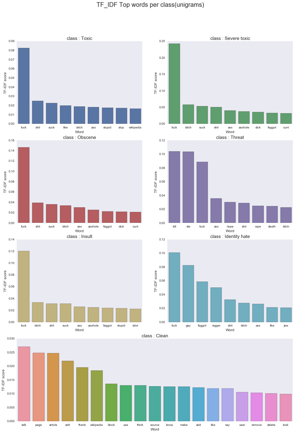
Most frequent toxic words
If interested, Jagangupta’s brilliant kernel explores the dataset in depth and presents a detailed report.
Text pre-processing
Little text pre-processing helped improve the results somewhat in the range of ~0.0005 mean ROC AUC (more on evaluation later). Replacing IP addresses by a token, replacing abbreviations, emojis and expressions such as “gooood” with appropriate/normalized words helped. Removing stop-words seemed to be hindering sequence models than helping them, which means models have been able to use at least some of the words. I also kept few symbols such as “!” and “?” since both fastText and GloVe embeddings have representations for symbols.
def clean(comment):
    """
    This function receives comments and returns a clean comment
    """
    comment=comment.lower()
    # normalize ip
    comment = re.sub("\d{1,3}\.\d{1,3}\.\d{1,3}\.\d{1,3}"," ip ", comment)
    # replace words like Gooood with Good
    comment = re.sub(r'(\w)\1{2,}', r'\1\1', comment)
    # replace ! and ? with ! and ? so they can be kept as tokens by Keras
    comment = re.sub(r'(!|\?)', " \\1 ", comment)

    #Split the sentences into words
    words=comment.split(' ')

    # normalize common abbreviations
    # replacements is a dictionary loaded from https://drive.google.com/file/d/0B1yuv8YaUVlZZ1RzMFJmc1ZsQmM/view
    words=[replacements[word] if word in replacements else word for word in words]

    clean_sent=" ".join(words)
    return(clean_sent)
Another interesting point is the maximum number of features used: it stops having any noticeable effect after a certain threshold. So to save the computation cost and time, it’s worth setting a limit. In Keras tokenizer, this can be achieved by setting the num_words parameter, which limits the number of words used to a defined n most frequent words in the dataset. In this case, I settled for 100,000 as the maximum number of words used for models.
It is same with the length of features used to represent a sentence, and can be selected by looking at the following graph.
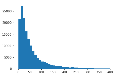
Number of words in a sentence. Source: https://www.kaggle.com/sbongo/for-beginners-tackling-toxic-using-keras
Sentences longer than a given threshold need to be truncated while shorter sentences need to be padded to fit the length. This is required before feeding a dataset to a sequence model because the model needs to have a defined number of units. In all experiments detailed, I used 200 as the sequence length as it didn’t have any noticeable difference using more features.
from keras.preprocessing import text, sequence

maxlen = 200 # length of the submitted sequence
EMBEDDING_FILE = './data/fasttext/crawl-300d-2M.vec'

train = pd.read_csv('../data/train.csv')
test = pd.read_csv('../data/test.csv')

x_train = train["comment_text"].fillna("fillna").values
x_test = test["comment_text"].fillna("fillna").values

# default filters parameter removes symbols ! and ? which we want to keep
tokenizer = text.Tokenizer(num_words=max_features, filters='"#$%&()*+,-./:;<=>@[\\]^_`{|}~\t\n')
tokenizer.fit_on_texts(list(x_train) + list(x_test))
x_train = tokenizer.texts_to_sequences(x_train)
x_test = tokenizer.texts_to_sequences(x_test)

# pad sentences to meet the maximum length
x_train = sequence.pad_sequences(x_train, maxlen=maxlen)
x_test = sequence.pad_sequences(x_test, maxlen=maxlen)

# build a mapping of word to its embeddings
def get_coefs(word, *arr): return word, np.asarray(arr, dtype='float32')
embeddings_index = dict(get_coefs(*o.rstrip().rsplit(' ')) for o in open(EMBEDDING_FILE))

# build the embedding matrix
word_index = tokenizer.word_index
nb_words = min(max_features, len(word_index))
embedding_matrix = np.zeros((nb_words, embed_size))
for word, i in word_index.items():
    if i >= max_features: continue
    embedding_vector = embeddings_index.get(word)
    if embedding_vector is not None: embedding_matrix[i] = embedding_vector
Models
The evaluation of models was based on the mean column-wise ROC AUC. That is, averaging the ROC AUC score of each column.
Though I tried a number of models and variations, they can be roughly summarized to five models.
- Logistic regression model combining unigram, bigram and character level features with td-idf weighting
- LSTM/GRU based model with GloVe and fastText embeddings
- LSTM/GRU + CNN model with GloVe and fastText embeddings
- A deep CNN model
- Sequence layer with attention
This is each model in detail.
-
- Logistic regression
The final LR model was a combination of three sets of features extracted from two unigram, bigram td-idf weighted 10,000 most frequent words combined with a character level tokenizer of lengths 2 to 6 (highest 50,000 features). With a single cross validation split of 5% this model achieved a highest LB score of 0.9805.
from sklearn.feature_extraction.text import TfidfVectorizer
from sklearn.linear_model import LogisticRegression
from scipy.sparse import hstack

class_names = ['toxic', 'severe_toxic', 'obscene', 'threat', 'insult', 'identity_hate']

# unigram feature extractor
unigram_vectorizer = TfidfVectorizer(
    sublinear_tf=True, strip_accents='unicode',analyzer='word', ngram_range=(1, 1),
    use_idf=1, smooth_idf=True, stop_words='english', max_features=10000
)
unigram_vectorizer.fit(all_text) # all_text is concat of training and test text
train_unigram_features = unigram_vectorizer.transform(train_text)
test_unigram_features = unigram_vectorizer.transform(test_text)

bigram_vectorizer = TfidfVectorizer(
    sublinear_tf=False, strip_accents='unicode', analyzer='word', ngram_range=(2, 2),
    use_idf=1, smooth_idf=True, stop_words='english', max_features=10000
)

bigram_vectorizer.fit(all_text)
train_bigram_features = bigram_vectorizer.transform(train_text)
test_bigram_features = bigram_vectorizer.transform(test_text)

char_vectorizer = TfidfVectorizer(
    sublinear_tf=True, strip_accents='unicode', analyzer='char',
    stop_words='english', ngram_range=(2, 6), max_features=50000
)
char_vectorizer.fit(all_text)
train_char_features = char_vectorizer.transform(train_text)
test_char_features = char_vectorizer.transform(test_text)

train_features = hstack([train_unigram_features, train_bigram_features, train_char_features])
test_features = hstack([test_unigram_features, test_bigram_features, test_char_features])

for class_name in class_names:
    train_target = train[class_name]
    classifier = LogisticRegression(solver='sag')

    classifier.fit(train_features, train_target)
    submission[class_name] = classifier.predict_proba(test_features)[:, 1]
-
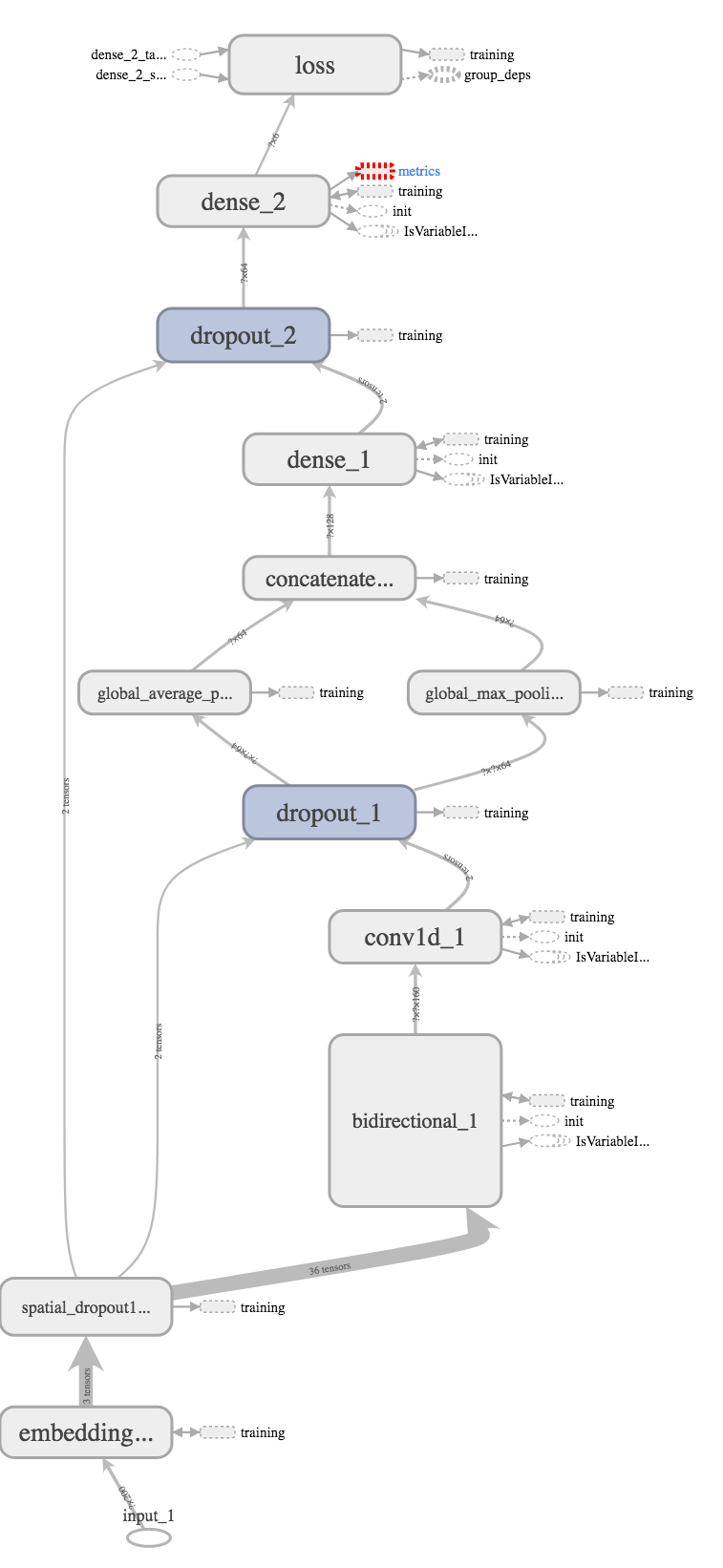
- A sequence model with bi-directional LSTM/GRU with embeddings
Essentially these are Bi-directional LSTM or GRU models taking embeddings as input. Initially I tried with a many-to-one model (returning only the last state) for the sequence layer, but this performed poorly. Influenced from the community, sequence layer was changed to return all states of units, and these time-distributed signals were captured by two pooling layers (average and max), and then concatenated and used as input for the final layer: six densely connected activation units (sigmoid) representing six output labels. This performed much better, achieving around 0.9830 on LB easily.
I tried few variations of the same model. Among them, a bi-directional LSTM/GRU layer connected to a time-distributed dense layer (figure a) and a multi-layer bi-directional LSTM/GRU model (figure b) are noteworthy. The multi-layer model seemed to be overfitting, and at best performed comparable to a single layer when regularized heavily with a high dropout rate. The single bidirectional LSTM layer connected to a time-distributed dense layer with a moderate dropout rate, however, performed a little better than a single bidirectional LSTM layer. So this last model was used for further model averaging.
One observations from this experiment was that it didn’t have much difference in accuracy whether it was LSTM or GRU units were used for the sequence layer. However, different embeddings had a noticeable difference. I tried with fastText (crawl, 300d, 2M word vectors) and GloVe (Crawl, 300d, 2.2M vocab vectors), and fastText embeddings worked slightly better in this case (~0.0002-5 in mean AUC). I didn’t bother with training embeddings since it didn’t look like there was enough dataset to train. This lecture explains what might happen when trying to train pre-trained embeddings on a small dataset.
For building models, Keras was used with default Tensorflow backend. As for the hardware, AWS P2 instances (Tesla K80 GPUs) were used.
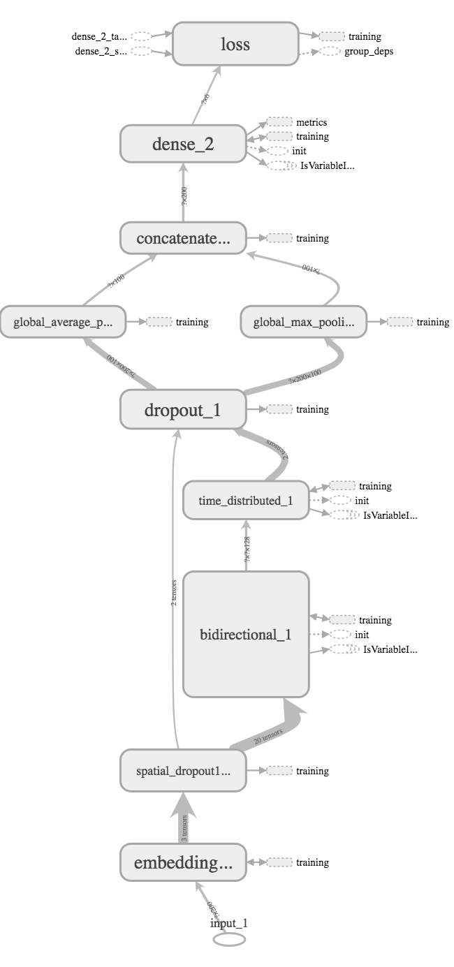 a) LSTM-Dense-Pooling |
 b) Multi-layer Bi-GRU |
def build_model(): # figure (a) as a Keras model
    inp = Input(shape=(maxlen, ))
    x = Embedding(max_features, embed_size, weights=[embedding_matrix])(inp)
    x = SpatialDropout1D(0.4)(x)
    x = Bidirectional(LSTM(64, return_sequences=True, recurrent_dropout=0.0, dropout=0.2))(x)
    x = TimeDistributed(Dense(100, activation = "relu"))(x) # time distributed  (sigmoid)
    x = Dropout(0.1)(x)

    # global pooling layer
    avg_pool = GlobalAveragePooling1D()(x)
    max_pool = GlobalMaxPooling1D()(x)
    conc = concatenate([avg_pool, max_pool])
    outp = Dense(6, activation="sigmoid")(conc)

    model = Model(inputs=inp, outputs=outp)

    return model

model = build_model()
opt = Nadam(lr=0.001)
model.compile(loss='binary_crossentropy', optimizer=opt, metrics=['accuracy'])
model.summary()
-
- LSTM/GRU + CNN model with GloVe and fastText embeddings
This model is an attempt at combining sequence models with convolution neural networks (CNNs). At the beginning I tried a convolution layer passing signals to the sequence layer. But it seems swapping these layers — embeddings feeding to LSTM first and then using a CNN on each LSTM unit’s state — and pooling to an output layer brings better results. This study and kernel better explain this model.
CNN-LSTM-pooling model
def build_model(): # figure (a) as a Keras model
    input = Input(shape=(maxlen, ))
    x = Embedding(max_features, embed_size, weights=[embedding_matrix])(input)
    x = SpatialDropout1D(0.4)(x)
    x = Bidirectional(LSTM(80, return_sequences=True, recurrent_dropout=0.2, dropout=0.2))(x)
    x = Conv1D(filters=64, kernel_size=2, padding='valid', kernel_initializer="he_uniform")(x)
    x = Dropout(0.2)(x)

    avg_pool = GlobalAveragePooling1D()(x)
    max_pool = GlobalMaxPooling1D()(x)
    conc = concatenate([avg_pool, max_pool])

    output = Dense(64, activation="relu")(conc)
    output = Dropout(0.1)(output)
    output = Dense(6, activation="sigmoid")(output)

    model = Model(inputs=input, outputs=output)
    return model
As a variation, I tried to emulate bigrams and trigrams using kernel sizes of 2 and 3 in the CNN layer and concatenating their outputs through pooling layers. But again, this seemed to overfit.
-
- A deep CNN model
This model is based on this paper and this kernel. In summary, it consists of multiple layers of convolution and pooling layers with skip layer connections. Unfortunately, this didn’t perform up to the mark of above two models, both fastText and GloVe embeddings scoring 0.9834 and averaging to 0.9843 on LB. It could be either due to not being able to spend time on tuning it or overfitting again. Still this could work with more data, and indeed, it has according to stats reported in the paper.
-
- Sequence layer with attention
This was a half hearted attempt. But still I wanted to try out how well attention works out. I used an attention layer and a secondary LSTM layer. Strangely, it couldn’t surpass the first two models without attention. Probably, it could have with more time spent on tuning it, but the training time needed was higher than other models.

Attention with LSTM (Source: https://www.coursera.org/learn/nlp-sequence-models/)
Model averaging and ensemble
Due to the relatively small dataset size, there seemed to be a case of overfitting. So it’s not surprising that model averaging and regularization showed a strong positive effect on the prediction accuracy. It was done through various forms: one was through stratified 10-fold training, and this improved the performance noticeably, though obviously it took more time. When averaging folds, weighted average or ranked average performed slightly better than taking the mean of predictions.
Another interesting tidbit is how to use stratified-k fold with multi label classification, since popular stratified k-fold scikit-learn function only supports single label splits. Here, numpy.packbits can come in handy.
import numpy as np
from sklearn.model_selection import StratifiedKFold

pred = np.zeros((x_test.shape[0], 6))
y_packed = np.packbits(y_train, axis=1)

kfold = StratifiedKFold(n_splits=10, shuffle=True, random_state=32)

for i, (train_idx, valid_idx) in enumerate(kfold.split(x_train, y_packed)):
    print("Running fold {} / {}".format(i + 1, n_folds))
    print("Training / Valid set counts {} / {}".format(train_idx.shape, valid_idx.shape))

    # train the model
Model averaging was done again using different embeddings: here, the predictions produced by the same model using GloVe and fastText embeddings were averaged. This step improved the final accuracy of predictions significantly: the best single LSTM-CNN model achieved 0.9856 on LB after averaging predictions from two embeddings, where GloVe and fastText only got 0.9850 and 0.9854 respectively using the same model.
Towards the end, the competition turned into an ensemble madness. I would have liked to try some stacking, which in my opinion is the better way of combining models than by randomly conjured up coefficients.
Improvements and notes from the community
In my opinion, the best feature of Kaggle competitions is the collaborative learning experience. Here are some of the effective techniques that have been used by other teams.
-
- Augmenting the train/test dataset with translation
Using translations is an interesting method of augmenting the dataset, and it has worked wonderfully without information leaking. The technique is quite simple: translate sentences to few nearby languages, and then translate them back to English. When you think about it, this makes sense since it can help reduce overfitting by adding more data with variations in the sentence structure. More details can be found from this kernel.
-
- Adding more embeddings
It seems much of the complexity in this case comes from the embedding layer; and using more embeddings helps more than using different structures. So using all variations of GloVe, Word2vec, LexVec and fastText (e.g., Crawl, Twitter, Wikipedia) can help by averaging resulting predictions. More on various pre-trained embeddings can be found from here and here.
-
- Byte-pair encoding (BPE)
Usually in any text processing work there is a large number of out of vocabulary words. In other words, these are the words that are not found in the embeddings. The standard way of handling such words is to use a token such as <unk> and moving on. Byte-pair-encoding has shown better results handling these kind of words by breaking the word into subwords — similar to phoneme in speech recognition — and using embeddings of these subwords to arrive at the full word. More on this can be found from here.
-
- Capsule networks
Few teams had tried Geoffrey Hinton’s Capsule Networks, and they have reported to be overfitting. Anyway, it’s something worth trying out.
Useful resources:
- Andre Ng’s Coursera Sequence models course – https://www.coursera.org/learn/nlp-sequence-models/. This is a cool course with lots of real world cases as project assignments, ranging from text generation, translations to trigger word detection. I’d recommend it to anyone interested in sequence models, having completed it myself.
- Word embedding trends – http://ruder.io/word-embeddings-2017/index.html
- 1st place solution – https://www.kaggle.com/c/jigsaw-toxic-comment-classification-challenge/discussion/52557
- Google Colab for free GPU processing – https://colab.research.google.com/